Sequential Testing at Booking.com

Reliable and fast product decisions

Introduction

At Booking.com, we apply AB testing in order to assess whether a change on our website or mobile application positively affects the customer experience. AB testing is a way of measuring the causal impact of the product change on a certain outcome, such as the conversion rate or click through rate. We randomly assign our customers to one of two groups: The group that sees the website unchanged and the group that sees the product change. The random assignment ensures that only the influence of the product change distinguishes the two groups and the influence of all other variables on the outcome is not systematic. This allows us to conclude that the observed difference between the groups was indeed caused by the product change.

We analyse the results with a statistical test that leads to one of two possible business decisions: the product change had a positive effect and will be shipped, or it did not and will not be shipped. Statistical tests control how often an ineffective change will wrongly be shipped (Type I or alpha error) and how often an effective change will be dismissed (Type II or beta error). Most often, hypothesis testing is done by calculating how much data is needed to reach a decision, given a pre-specified alpha and beta error rate and a minimal relevant effect size. This calculation needs to be done upfront and requires waiting until sufficient data has been collected (so-called fixed horizon testing). In practice, it is hard for experimenters not to look at interim results for a faster decision. Crucially, not adhering to the runtime increases the alpha error. A major benefit of sequential testing is that it does allow for interim analyses while maintaining the correct alpha error rate.

Interestingly, the upfront calculation also requires a judgment call: How much of an impact on the customer is worth our efforts? We refer to this number as the minimum relevant effect or in short MRE. The calculation of the sample size is based on the MRE, which is informed by the team’s previous experiments, business targets and a definition of success. Ideally, costs and benefits can be weighed against each other to judge the optimal MRE. In practice however, this is a very complex calculation and many times considerations beyond pure cost-benefit trade offs enter the equation as well. Thus, it is quite likely that the choice of the MRE is a bit arbitrary. In addition, the real impact of the product change might be substantially larger than this MRE, rendering the calculated sample size substantially too large for its purpose. Such misestimation affects the product community and the business in crucial ways by wasting valuable time and resources. Mainly since once the AB experiment runs, the product managers have to wait for the pre-determined sample size before they can make a decision. This is problematic for two possible reasons:

1. If they see promising signals early on during the runtime, they cannot act on them without substantially increasing the false positive rate. Due to the arbitrary nature of the MRE, an early signal is likely whenever the real impact exceeds the MRE sufficiently.
2. When the real impact is a lot smaller than the MRE, the AB experiment runs until the required sample size arrives, all the while showing virtually no impact or an impact way too small to be relevant.

In both scenarios it leads to a waste of valuable time. Experimenters have to wait for the result of a test that is either doomed to show failure or could declare success a lot earlier.

The solution to this problem are methods that allow for intermediate opportunities to judge the outcome of the test and act accordingly. This concept of sequential testing goes back to Wald (1945) and was adapted to clinical research by Armitage et al. (1969). Pocock (1977, 1982) and O’Brien and Fleming (1979) developed the group sequential design (GSD) which is the main focus of this article. GSD is widely used in clinical and pharmaceutical research for obvious reasons: early stopping requires fewer patients and allows for applying the better treatment to as many patients as possible as early as possible and prevents further patients experiencing serious adverse events if there is a strong safety issue.

However, it largely remains underutilised in other parts of academia and industry alike. We will argue that they are very well suited for most business needs and compare favourably to alternative methods.

Overview of common sequential tests

In this section, we will give an overview of existing methods that are often mentioned as possible alternatives to the Group Sequential Design . As we will see, they all have different use cases and objectives. Thus, different business objectives require different methods. Our use case in Booking.com and the use cases of many other online companies however, are perfectly suited for Group Sequential Design, for theoretical as well as practical reasons.

Adaptive Bandits

Bandit methods generally have a different goal than hypothesis tests. The main idea of bandits is to sacrifice some exploration in favor of exploitation (Gittins, 1979, Robbins, 1952). This shifts the goal from reaching a valid statistical conclusion in an optimal amount of time to using information gained during the experiment to increase traffic for the best performing variant(s) and reap its benefits already during the runtime. A classic example is a performance comparison of different headlines for an online news article. In this scenario, the readers will likely lose interest after merely a few days and there is no need for confidence intervals and/or controlling false positive rates. It suffices to determine the best version with sufficient probability and allocate more traffic to the variants that maximise click-through rates.

In settings where the objective is a valid statistical conclusion, bandits perform suboptimally in terms of the sample sizes they need. Moreover, adaptive bandits suffer from systematic bias (Nie, 2017). Variants with too optimistic point estimates will get more traffic while variants with too pessimistic point estimates will get less traffic. Thus, sampling errors directly affect the data collection and sampling errors do not cancel each other out anymore.

Always valid p-values

In an effort to be able to monitor results continuously without sacrificing the validity of the confidence intervals and control the false positive rate, always valid p-values (Lindon et al., 2022, Ramesh et al., 2019) are a viable alternative. Always valid p-values can achieve a favourable tradeoff between power and run-time. In this article, we will consider the mixture sequential probability ratio test (mSPRT, called sprt for brevity) which is used by Optimizely, Uber, Netflix, and Amplitude.

It allows users to continuously monitor experiments and derive inferences at any time without even specifying a maximum sample size. While this is certainly an extremely powerful testing framework, in most practical applications specifying a maximum sample size is beneficial. In fact, in virtually all cases we have encountered at Booking.com, product teams wish to know the time they have to wait until valid statistical results allow for a decision. Following Spotify and their excellent blogpost, we also consider a more general method of always valid p-values (Howard et al., 2022), the so-called generalisation of always valid inference (gavi) that is currently used by Eppo.

Always valid p-values have correct statistical properties and possess the nominal coverage property of the corresponding confidence intervals. A subtle aspect that often gets overlooked, though, is that they don’t necessarily provide a valid decision making procedure. This goes back to two reasons:

• The alpha error is only correct if the user stops the experiment the very moment the confidence interval excludes 0 for the first time.
• Furthermore, even though those tests eventually provide a power of 1 with increasingly large sample sizes, this isn’t a meaningful property, since any valid imaginable test provides arbitrarily high power with large samples. However, sample size can never be seen as an infinite resource. Thus, for any finite sample size, there is effectively no power control.

Ad-Hoc analysis

Some companies, such as Statsig (StatSig 2023), use a simple adjustment that inflates the standard error proportional to the sample size that has already arrived. The smaller the sample size, the larger the standard error. This partially reduces the increase of false positives of this sequential analysis compared to a naive reading of a fixed horizon test at each interim analysis. However, it lacks a systematic approach and alpha depends on the specific setup.

Group Sequential Design

The focus of this article is on Group Sequential Designs (GSD), a variant of repeated significance testing. At the core of this method lies the concept that error rates are a resource to be spent throughout the experiment, according to a pre-defined function (error-spending functions, Lan and DeMets 1983). Its idea is to specify a proportion of the desired significance level that is spent up to an interim checkpoint, which has many advantages over the alternative of directly specifying the form of the adjusted significance levels. The most important is that the sample size per checkpoint, and even the exact number of checkpoints, doesn’t need to be known in advance. All that is needed is to specify the maximum sample size at which the experiment stops (Lakens, 2021). Error-spending functions can define one or two decision bounds, an upper bound and a lower bound. When the test statistic exceeds the upper bound, the null hypothesis can be rejected. When the test statistic falls below the lower bound, the experiment can stop for futility and we accept the null hypothesis. Group Sequential Designs offer the choice of using binding bounds (Wassmer, 2016), whereby once a bound has been crossed the decision is final. Non-binding bounds would offer the option to keep the experiment running, and potentially reverse the decision later. In the business context, a binding bound is desirable, since this offers a clear and well defined decision framework with no wiggle room. Furthermore, it offers clear expectations about the average and maximum duration. This is particularly attractive for online experimentation where daily checkpoints, rather than checkpoints specified by exact sample sizes, are a natural choice.

GSD also allows for the calculation of valid confidence intervals (Wassmer, 2016). Two fundamentally different ways of getting precise confidence intervals exist. One method only enables the calculations after the experiment has been completed and requires adherence to the predefined stopping rules. This method is referred to as final confidence intervals (Wassmer, 2016). The other method only considers how much the statistical errors are being inflated due to the number of additional checkpoints. These are so-called repeated confidence intervals and are still valid even if researchers decided to not stop an experiment at earlier checkpoints if they could (or should) have done so. This is particularly attractive in the context of clinical trials, where the collection of additional data in combination with valid confidence intervals might be necessary. For example if a particular drug has been shown to have significant benefits early on that need to be quantitatively monitored or if there are still valuable learnings to be gathered about one of multiple endpoints.

Empirical comparison

The empirical comparison entails the following methods:

• Group Sequential Design Test as used by Booking.com (gst)
• Group Sequential Design Test as used by Spotify (gst_spot)
• Generalisation of Always Valid Inference as used by Eppo (gavi)
• (Mixture) Sequential Probability Ratio Test as used by Optimizely, Uber, Netflix, and Amplitude (sprt)
• Simple ad-hoc alpha correction as used by StatSig (ss)

WE have simulated 1000 iterations of AB experiments. Every simulated AB experiment was analysed at different interim analyses using all 5 methods mentioned above and had 1000 visitors in the treatment and in the control group.

• gst and gst_spot were calculated at 5 interim analyses after every 200 new visitors
• gavi, sprt, and ss were calculated after each and every new visitor with as many interim analyses as possible (999, since there is no standard deviation after just 1 visitor in each group).

This setup was used in four scenarios with four different underlying treatment effects (0 or no effect, 0.09, 0.13, 0.17) using Gaussian data. Those correspond to powers of (5%, 64%, 90%, and 98%). Thus, in total 4000 AB experiments were analysed, each with each of the methods. In case of no effect, the 5% “power” of the experiment corresponds to the nominal false positive rate, alpha. we analysed

• False Positive Rate (a 5% false positive rate corresponds to 50 positive results among the 1000 simulated AB experiments)
• Power (a 80% true positive rate corresponds to 800 positive results among the 1000 simulated AB experiments)
• Required sample size (this is the sample size at which a method reached a definitive conclusion, i.e. the first time the confidence interval excluded 0)

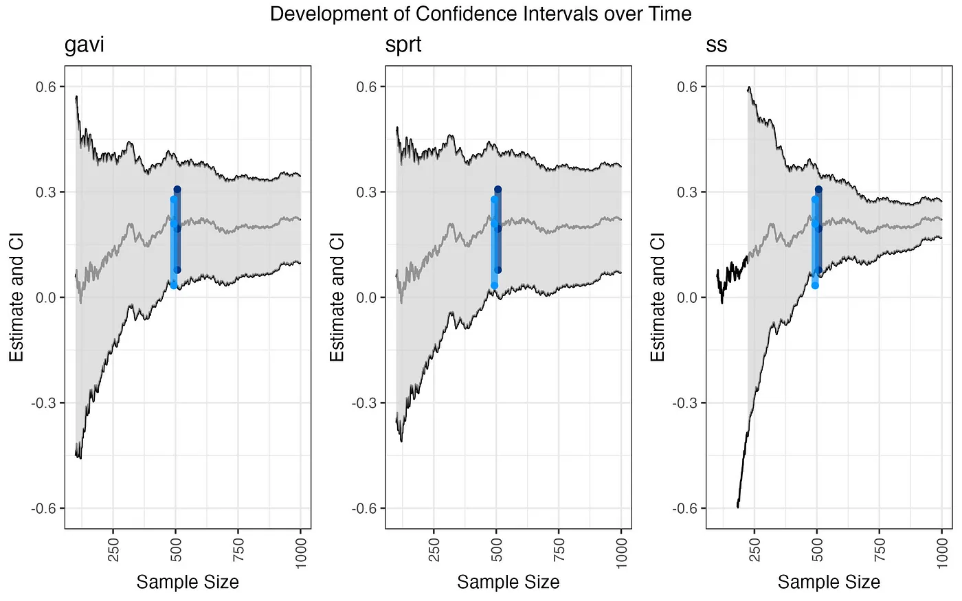
Before we dive into the results, take a look at the following picture (Figure 1), it shows the confidence intervals of the different methods over time. Depicted in dark blue is the final confidence interval of the group sequential design as used by Booking.com at decision time, and in light blue we see the final confidence interval as used by Spotify. We can see that both methods provide substantially smaller confidence intervals than the always valid methods. As mentioned above, the confidence intervals of group sequential designs provide the correct nominal coverage (Wassmer, 2016). The ad-hoc method (ss) shows that its confidence intervals are too wide in the beginning and too narrow in the end of the sequential analyses.

Figure 1. Confidence intervals of the different methods over time. Depicted in dark blue is the final confidence interval of the group sequential design as used by Booking.com at decision time, and in light blue we see the final confidence interval as used by Spotify. We can see that both methods provide substantially smaller confidence intervals than the always valid method. The ad-hoc method shows that its confidence intervals are far too wide in the beginning and too narrow in the end of the sequential analyses.

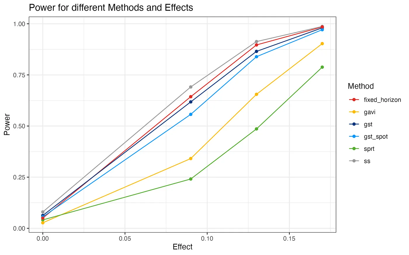
False positive rate and power

Group Sequential Design show by far the highest power (Table 1 and Figure 2). The GST method as used at Booking.com ends up almost on par with a fixed horizon test. The GST design that Spotify uses follows closely with a power that is about 6–8% lower for the two medium sized effects. The next two contesters, gavi and sprt show substantially lower power for all scenarios.

Table 1. Realised power (or false positive rate) for the different methods and effects. Note that the first row corresponds to the case where no real effect (difference between treatment and control group of the AB experiments) was present. Thus, the number should theoretically be 0.05 for all methods looked at, except for ss which doesn’t properly control for the false positive rate. The small deviations from the correct 0.05 value are sampling errors of the simulations and will average out to equal 0.05 in the long run.

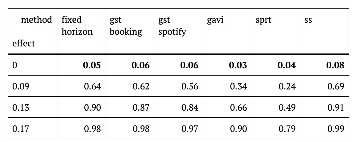
Interestingly, the ss method inflates the false positive rate to some degree and thus, the observed powers for this method aren’t directly comparable.

Figure 2. Power for four different effects and all Methods. Apart from ss which doesn’t show the correct false positive rate, gst as used by Booking.com shows power values that are closest to a fixed horizon test. Spotify’s gst is about 6–8% behind. Both always valid methods, gavi and sprt, have far lower power for all tested effects.

Sample size

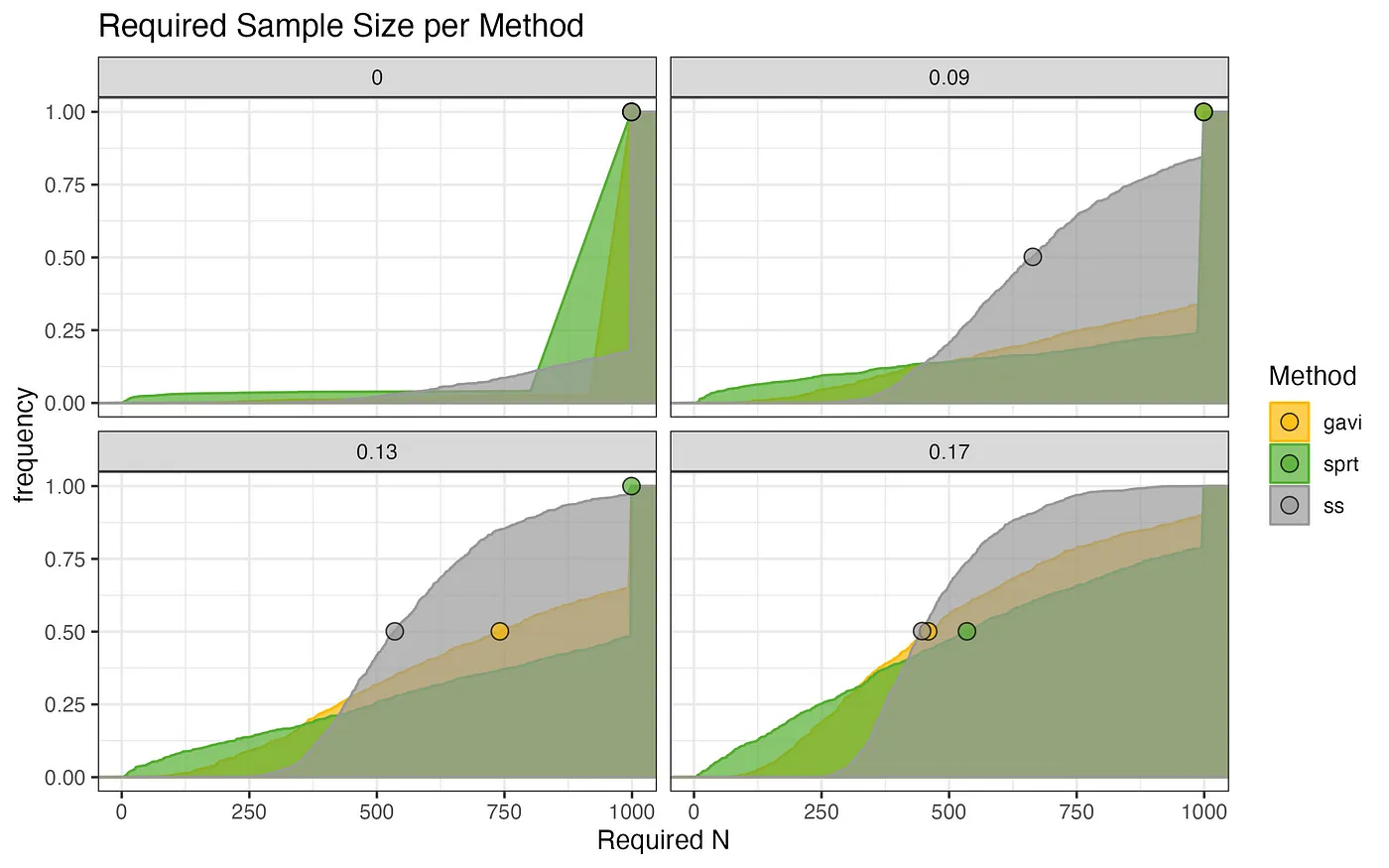
Figures 3 and 4 show the cumulative distribution of the required sample size to terminate the test on the x-axis and the frequency of occurrence on the y-axis. For a better visual impression, we have used a kernel density estimation to smooth the graph.

Figure 3. Cumulative densities of the required sample sizes per method and effect size. Median required sample sizes are indicated by points. Note that the median should correspond to 0.5 on the y-axis. The reason that it doesn’t always do this here is the smoothing effect of the density estimation, whenever there are different values possible that qualify as a median, the smoothing determines the exact y-values.

As shown in table 2, the method that terminates fastest is our implementation of gst. Particularly striking is its advantage compared to the other methods when looking at the almost uniform distribution (the cumulative density of a uniform distribution increases linearly) of sample sizes needed to stop an experiment early for futility, which is the case when the effect equals zero.

Table 2. Median required sample size to detect an effect for the different methods and effects.

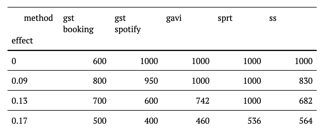
Given that in most contexts, interventions with no impact comprise the majority of experiments, this is a crucial advantage in terms of speed for the product development that you don’t get from any of the other methods. For the smaller effect size of 0.09, Booking.com’s gst terminates the fastest and shows the most desirable distribution of required sample sizes. For the two larger effects, Spotify’s method requires slightly smaller sample sizes in those cases where both methods detected the effects.

Figure 4. Cumulative densities of the required sample sizes per method and effect size. Median required sample sizes are indicated by points. Both gavi and sprt never stop early when no effect is present and substantially later for all three effects. The stopping times of ss are equally unsatisfying for no effect and show an early mode for the other three effects. Note that the median should correspond to 0.5 on the y-axis. The reason that it doesn’t always do this here is the smoothing effect of the density estimation, whenever there are different values possible that qualify as a median, the smoothing determines the exact y-values.

Summary

Group Sequential Designs are particularly well suited for situations where data arrives in batches, e.g. daily reports. In a business context, it is desirable to be able to put an upper bound on the runtime of an AB test. Since Group Sequential Designs are guaranteed to stop with a decisive result when a maximum sample size has arrived, they always enable a statistically valid conclusion within a planned duration. If on the other hand there is a need for analysing data in real time or analysing a certain product change for the indefinite future, methods that provide always valid confidence intervals are better suited for the task.

All valid statistical procedures investigated in this article (Booking’s gst, Spotify’s gst, gavi, sprt) provide correct control of false positive rates. StatSig’s ad hoc procedure does not guarantee a correct false positive rate. In terms of power and average required sample sizes, both group sequential designs outperform the other methods by a large margin. Booking’s design has the additional advantage of stopping early even in case of no effect.

Moreover, since setting the minimum relevant effect a priori is very hard, practical advantages of sequential tests over fixed horizon tests are even larger than merely evaluating the efficacy of sequential tests by their false positive rates and statistical power. Fixed horizon tests are only correctly powered in case the impact for which the test was designed is exactly correct. Otherwise, the test could either have done well with a much smaller sample size or was a hopeless endeavour from the get go. We have seen that the group sequential design as used by Booking.com saves valuable product development time in the majority of cases where the product change has no substantial impact. Thus, Group sequential tests greatly improve reliability and speed of our product development cycles.

Correction

A previous version of this article reported incorrectly 0.18 as the false positive rate for ss. The correct number is 0.08. This was due to a mistake in the code. The numbers for the corresponding powers have also been corrected. Since then StatSig has revamped their Sequential Testing method. Their new approach has improved statistical power while enforcing correct false positive rates.

References

Armitage, P., McPherson, C. K., & Rowe, B. C. (1969). Repeated significance tests on accumulating data. Journal of the Royal Statistical Society A, 132, 235–244.

Gittins, J. C. (1979). Bandit Processes and Dynamic Allocation Indices. Journal of the Royal Statistical Society. Series B (Methodological). 41 (2): 148–177. doi:10.1111/j.2517–6161.1979.tb01068.x. JSTOR 2985029. S2CID 17724147.

Howard, S. R., Ramdas, A., McAuliffe, J., Sekhon, J.(2022). Time-uniform, nonparametric, nonasymptotic confidence sequences. arXiv 1810.08240

Lakens, D., Pahlke, F., & Wassmer, G. (2021). Group Sequential Designs: A Tutorial.

Lan, K. K. G., & DeMets, D. L. (1983). Discrete sequential boundaries for clinical trials. Biometrika, 70, 659–663.

​​Lindon, M., Ham D. W., Tingley M., Bojinov, I.(2022). Anytime-Valid F-Tests for Faster Sequential Experimentation Through Covariate Adjustment. arXiv 2210.08589

Nie X., Tian X., Taylor, J., Zou J. ( 2017). Why Adaptively Collected Data Have Negative Bias and How to Correct for It. arXiv:1708.01977

O’Brien, P. C., & Fleming, T. R. (1979). A multiple testing procedure for clinical trials. Biometrics, 35, 549–556.

Pocock, S. J. (1977). Group sequential methods in the design and analysis of clinical trials. Biometrika, 64, 191–199.

Pocock, S. J. (1982). Interim analyses for randomized clinical trials: The group sequential approach. Biometrics, 38, 153–162.

Ramesh J., Pekelis L., Walsh D. (2019). Always Valid Inference: Continuous Monitoring of A/B Tests. arXiv: 1512.04922

Robbins, H. (1952). Some aspects of the sequential design of experiments. Bulletin of the American Mathematical Society. 58 (5): 527–535. doi:10.1090/S0002–9904–1952–09620–8.

StatSig (2023). Documentation about Sequential Testing.

Wald, A. (June 1945). Sequential Tests of Statistical Hypotheses. Annals of Mathematical Statistics. 16 (2): 117–186.

Wassmer, G., Brannath, W. (2016). Group Sequential and Confirmatory Adaptive Designs in Clinical Trials. Springer Series in Pharmaceutical Statistics.

Acknowledgments

Kostas Tokis , Sam Clifford, Guy Taylor, and Kelly Pisane provided invaluable feedback during the writing of this article.